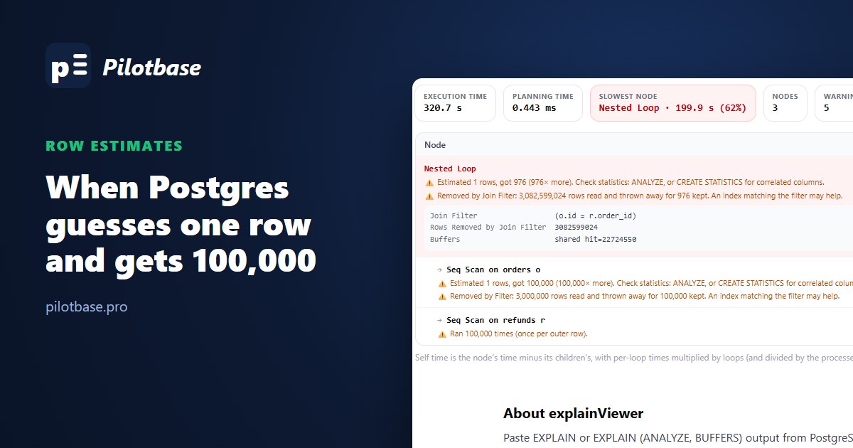
The query joins last night's orders to their refunds. It ran in 5 minutes and 21 seconds. We changed nothing in the query, added no index, touched no setting, ran one command that took a tenth of a second, and it ran in 181 milliseconds.
The command was ANALYZE orders. The query had been planned for one row and got a hundred thousand.
Almost every Postgres plan that is absurdly slow, as opposed to merely slow, has this shape: somewhere near the bottom the planner believed in a handful of rows, chose a method that's perfect for a handful, and reality delivered thousands of times more. This article produces that failure four different ways on PostgreSQL 18, with the plans, and fixes each with the tool made for it: ANALYZE, CREATE STATISTICS on columns, CREATE STATISTICS on an expression, and the statistics target.
Where the guess comes from
Postgres never looks at your data while planning. It looks at a summary that ANALYZE wrote into pg_statistic the last time it ran: for each column, the share of NULLs, the number of distinct values, the hundred most common values with their frequencies, and a histogram of the rest. ANALYZE builds that from a random sample, 30,000 rows per table at default settings, however big the table is.
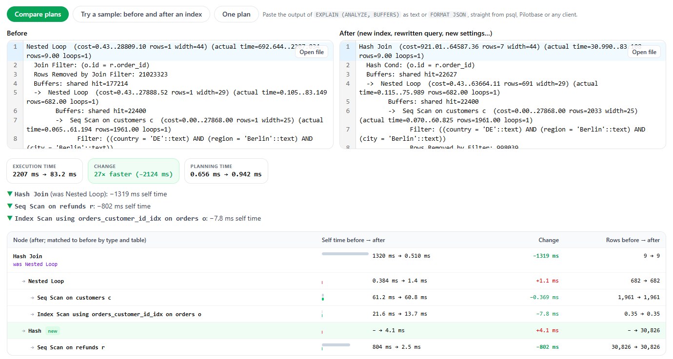
From the summary the planner works out, for every step of every candidate plan, how many rows will come out. That number is the rows= in EXPLAIN. With EXPLAIN ANALYZE you get the real count next to it, and comparing the two, from the innermost node outwards, is the whole diagnostic method. The first node where they part ways by 10x or more is where to look. explainViewer does the comparison for you and flags those nodes.
Our test database is a shop: 1,000,000 customers in 1,200 cities, 3,000,000 orders loaded in thirty nightly imports of 100,000, and a refunds table of about 30,000 rows that is new enough that nobody has indexed its order_id yet.
Case 1: the load nobody analyzed
Night 31. The import job adds 100,000 orders with import_id = 31, and a report asks for their refunds:
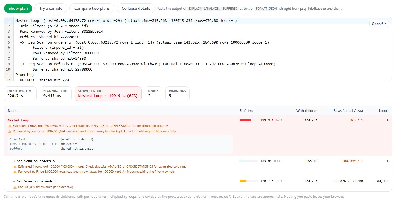
Read it from the bottom. Seq Scan on orders: estimated 1 row, actual 100,000. Everything above follows from that. For one order, the cheapest way to find its refunds is to read the small refunds table once, so the planner picked a Nested Loop over a sequential scan. For 100,000 orders it read that table 100,000 times, compared 3,082,599,024 pairs of rows and kept 976.
Why one row? The statistics on orders were written when the table had thirty imports. All thirty values of import_id are in the most-common-values list, and their frequencies add up to 100%. A thirty-first value has no room to exist, so the estimate is the minimum the planner ever uses: 1. Ask for import 30 and it says 105,076, which is about right.
And why hadn't autovacuum fixed it? It analyzes a table when the rows changed since the last analyze pass a threshold:
A nightly load of 100,000 rows is a third of that. It takes more than three such nights to cross the line, and until then every query on the newest imports is planned as if they weren't there. The bigger the table grows, the longer the newest data stays invisible. (For this test we switched autovacuum off on the table so that the run repeats exactly; with the default settings it would not have fired either.)
The fix is one line at the end of the load job:
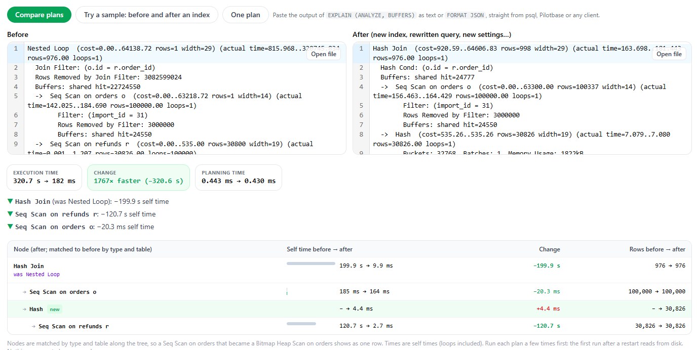
The estimate is now 100,337, the planner builds a hash table from refunds and probes it, and the query takes 181 ms. Three notes before moving on.
If you can't put ANALYZE in the job, lower the threshold for that table: ALTER TABLE orders SET (autovacuum_analyze_scale_factor = 0.01) makes autovacuum analyze it after about 30,000 changed rows. It still runs up to a minute behind the load.
Some tables autovacuum never analyzes. Temporary tables (it can't see them), foreign tables, and the parent of a partitioned table. A multi-step report that fills a temp table and then joins it is this same bug in miniature, and an ANALYZE after the fill is the cure. For bulk loads from files in general, see A messy CSV into Postgres without surprises.
Yes, an index on refunds.order_id would have rescued this query. Add it. But the estimate would still be wrong, and the next query that filters on the newest import and joins to something larger would go the same way. Fix the estimate first; then see which indexes you still need.
Case 2: columns that say the same thing
Now statistics that are perfectly fresh and still wrong. Every customer has a country, a region and a city, and the planner knows each column well:
Put the conditions together, the way an application with a country, region and city filter does:
The planner multiplies. 9.7% of customers are in Germany, 0.19% are in Berlin, so 0.018% are in both. That would be right if city and country had nothing to do with each other. But everyone in Berlin is in Germany; the second condition removes nobody. Each redundant condition divides the estimate again, and with three of them it hits the floor of 1.
One row, a join, and a table with no index on the join column. The same trap as before, sprung by different means:
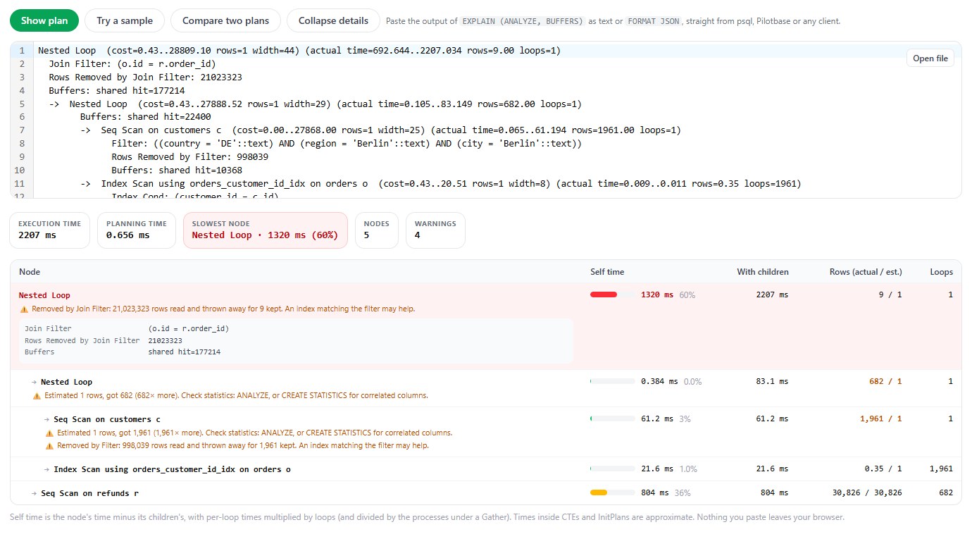
ANALYZE won't help here. It collects statistics per column, and no per-column statistic can say that one column decides another. For that you tell Postgres which columns belong together:
The three words in the brackets are three different kinds of knowledge, and it's worth knowing which one did the work.
dependencies records how strongly one column determines another. Ours, read back from pg_stats_ext: city decides country (1.0), city decides region (1.0), region decides country (1.0), region decides city only weakly (0.04). With that alone the Berlin estimate went from 1 to 1,733. It's tiny and cheap, and it has a blind spot the documentation spells out: it assumes the values you ask for are compatible. country = 'FR' AND city = 'Berlin' matches nobody, and with dependencies alone the planner estimated 1,733 for that too, where plain statistics had said 130. It also only applies to = and IN against constants.
mcv stores the most common combinations of values with their real frequencies, 100 of them by default. That's what brought Berlin to 2,033 and New York (39,681 customers) from an estimate of 360 to 37,900. It also pulled the impossible France-and-Berlin combination back down to 147. It costs more to build and to plan with, so keep it for columns that really are filtered together.
ndistinct counts distinct combinations, which matters for GROUP BY. Before, GROUP BY country, region, city was estimated at 100,000 groups; after, 1,200, which is exactly right. That estimate decides how much memory a HashAggregate plans for and whether it sorts instead.
Is every wrong estimate worth this? No, and the same table shows it. Before the statistics object existed, the New York version of the query was estimated at 360 customers and got 39,681, a miss of 110x, and it still ran in 227 ms on a sensible plan. At 360 rows the planner already preferred a hash join; being wrong didn't move it across a decision. Berlin was wrong by more and, crucially, wrong all the way down to 1. An estimate of rows=1 on a node that feeds a join is the one to hunt.
The cost side, measured: ANALYZE customers took 0.16 s before and 0.47 s with the three-column object. The documentation's advice is to create these for column groups that are used together and produce bad plans, not for every pair you can think of.
Case 3: a function around the column
Statistics describe columns. Wrap the column in a function and the planner has nothing to look up, so it falls back on constants that are compiled in: an equality matches 0.5% of the table, an inequality matches a third.
Every number in the left column is 0.5% or 33.3% of the table. None of them has anything to do with the data. Three ways out, best first.
Leave the column bare. A day is a range, and the planner has a histogram for ranges:
It's also the only form that can use an ordinary index on created_at. Likewise amount > 590 / 1.2.
Statistics on the expression. When the function has to stay, PostgreSQL 14 and later can collect statistics for the expression itself, without the cost of maintaining an index:
The expression has to match what the query says. After those three, created_at::date = '2026-09-14' was still estimated at 15,500: a cast to date is a different expression from date_trunc, and nobody collected anything for it.
An expression index, if you need the index anyway. CREATE INDEX ON customers (lower(email)) gets statistics for lower(email) at the next ANALYZE as a side effect. Don't build an index only for its statistics; that's what the previous option is for.
Case 4: more values than the list can hold
The most-common-values list has 100 entries per column by default (default_statistics_target). Our city column has 1,200 values. The top 100 get their real frequencies; the other 1,100 share what's left equally:
The same estimate for both, because to the planner they're the same: "some city not on the list". Here that's harmless. It stops being harmless when the tail is uneven, a few thousand customers with ten orders each and one account with two million. Raise the target for that one column:
It isn't free, and it's less free than it looks. The sample size follows the highest target on the table, and extended statistics are built from that larger sample too: with city at 1000 and the statistics objects from cases 2 and 3 in place, ANALYZE customers took 8 seconds, against 0.16 s for the plain table. Raising default_statistics_target to 1000 for every column, without any extended statistics, took 1.76 s. Bigger lists also make every plan that touches the table a little slower to produce. One column at a time, where a plan proves it's needed.
The same sample is why the number of distinct values is often low on big tables. For orders.customer_id Postgres estimated about 736,000 distinct customers; the real number is 955,195. You can't count distinct values reliably from 30,000 rows out of three million. If a GROUP BY or a join estimate suffers from it, tell Postgres the answer: ALTER TABLE orders ALTER COLUMN customer_id SET (n_distinct = -0.31) (negative means a fraction of the row count, so it stays right as the table grows). After the next ANALYZE our estimate was 961,000.
A routine for the next slow plan
Get the plan with EXPLAIN (ANALYZE, BUFFERS) and find the lowest node where estimated and actual rows differ by 10x or more. Then ask, in this order:
Are the statistics old? SELECT relname, last_analyze, last_autoanalyze, n_mod_since_analyze FROM pg_stat_user_tables answers it. If the table was loaded, bulk-updated or created since, run ANALYZE and plan again before trying anything cleverer. This is the cause more often than the other three together.
Is there a function or a calculation around the column? Rewrite to a bare column if you can, expression statistics if you can't.
Are there two or more conditions on columns that move together? Country and city, product and category, status and a date that's only set in that status, a tenant and anything owned by it. CREATE STATISTICS on that group.
Is the value outside the top 100, in a column with a long uneven tail? Raise that column's statistics target.
Then run the query again and compare the two plans, not just the two times. You want to see the estimate come right at the node you fixed and the join method change above it. If the estimate is right and the plan is still slow, it was never an estimate problem, and you're back to indexes and query shape. And if it's a Sort on a text column that's eating the time, that's a different story: Sorting text in Postgres is slow.
Paste the plan into explainViewer: it marks every node where the estimate and the real row count part ways, shows how many times each node ran, and compares the plan before and after your fix. It runs in your browser; nothing is uploaded. Run the queries and the ANALYZE in Pilotbase.
Open explainViewerSources: PostgreSQL documentation, Statistics Used by the Planner (per-column and extended statistics, the limits of functional dependencies), CREATE STATISTICS (kinds, expression statistics), How the Planner Uses Statistics (worked row estimates), Routine Vacuuming (when autovacuum analyzes, and the tables it doesn't), ANALYZE and ALTER TABLE (SET STATISTICS, n_distinct). Every estimate, timing and plan is from our own run: PostgreSQL 18.6, 1,000,000 customers, 3,100,000 orders and 30,826 refunds, parallel query and JIT off; screenshots from explainViewer in Chrome.
Comments (0)
Loading comments…